Spatial features: the fundamentals

Spatial features from first principles

Early on my geospatial learning path I came across Barry Rowlingson’s cheat sheet for R’s sp and raster librarys. I find it really useful to build simple test examples from scratch to make sure I know what I’m doing before diving in to large data sets and being overwhelmed be multiple tricky edge cases (or worse, corner cases). Barry’s page helped with this, you can find it here.

I wanted to make something similar for the sf package. sf (spatial features) will eventually be the defacto method for geospatial computing in R (although sp will be around for a long time and the two packages play well together with a number of methods for converting data types between the two). For excellent full coverage of sf and geospatial programming in R see the free book by Lovelace et al.. The remainder of this post walks through making very simple spatial objects using the sf package.

Making a single point

All functions operating on spatial data in the sf package begin with st_ which stands for spatial type. Starting with the simplest spatial type: a single point, I specify a two element vector where the two values are the X and Y coordinates of the point.

single.point <- c(10, -2)
single.point.st <- st_point(single.point)
## Take a look at the description of this objects class:
class(single.point.st)
## [1] "XY"    "POINT" "sfg"

Making multiple points

I specify a table with two column. Each row is a point, and the columns are the X and Y coordinates.

multi.point <- rbind(c(10, -2),
                     c(11, -2),
                     c(11, -1),
                     c(10, -1))
multi.point.st <- st_multipoint(multi.point)
class(multi.point.st)
## [1] "XY"         "MULTIPOINT" "sfg"

A linestring

Here I encode the multi.point table as a linestring with the points connected in the order of the table rows.

linestring.st <- st_linestring(multi.point)
plot(linestring.st)

A multi line string.

multiline.st <- st_multilinestring(list(multi.point, multi.point + 1.5))
plot(multiline.st)

A polygon

A polygon begins and ends at same location:

closed.ring <- rbind(multi.point, multi.point[1, ])
polygon.st <- st_polygon(list(closed.ring))
plot(polygon.st)

A polygon with a hole

Place the various individual polygons in a list with the perimiter as the first element, the following elements are coords of inner holes.

polygon.hole.st <- st_polygon(list(closed.ring, rbind(c(10.2, -1.25),
                                                      c(10.8, -1.25),
                                                      c(10.8, -1.2),
                                                      c(10.2, -1.2),
                                                      c(10.2, -1.25))))
plot(polygon.hole.st)

Multi polygons

These are specified simply by making a list of polygons.

multi.poly.st <- st_multipolygon(list(list(closed.ring), list(closed.ring + 2)))
plot(multi.poly.st)

Multi-geometry object

These are created by placing multiple goemetries of any type into a list and calling st_geometrycollection.

Geometry columns

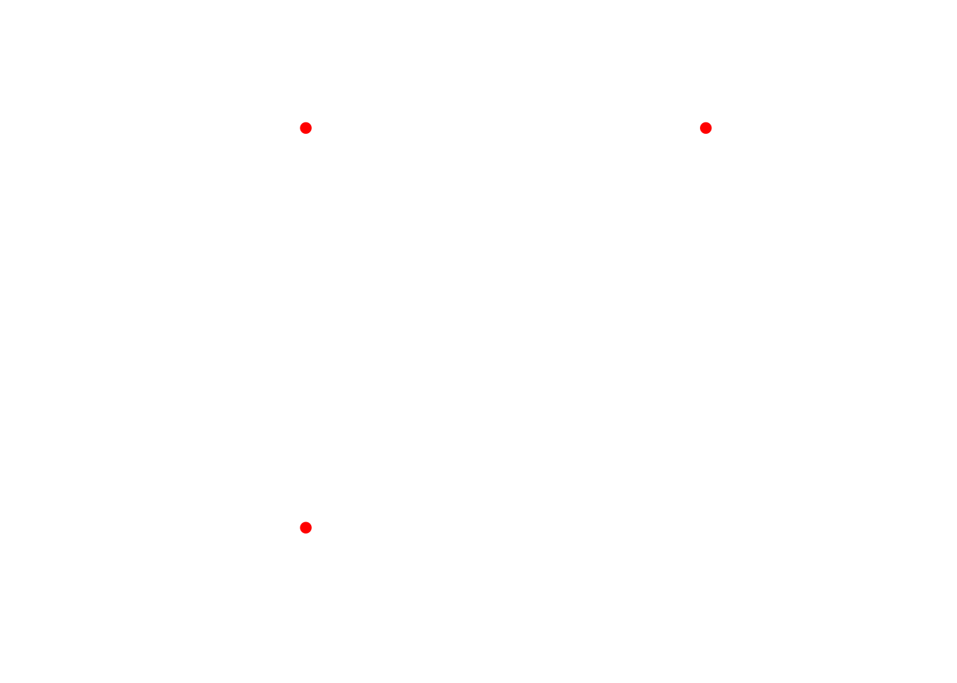
It’s really useful to be able to combine individual spatial feature geometries (sfg’s) into columns. These columns would usually be of the same type eg., all points or all polygons. Here, I’m making a spatial feature geometry column for three points.

points.sfc <- st_sfc(list(st_point(c(10, -2)), st_point(c(10, -3)), st_point(c(11, -2))))
plot(points.sfc, col="red", pch=19)

## To extract the coordinates into matrix form:
st_coordinates(points.sfc)
##    X  Y
## 1 10 -2
## 2 10 -3
## 3 11 -2

Adding a Coordinate Reference System (CRS)

I can do this either with a European Petroleum Survey Group (EPSG) code or directly with a proj4 character string.

points.copy <- points.sfc
st_crs(points.sfc) <- 4326 # EPSG code 4326 (WGS84)
print(points.sfc)
## Geometry set for 3 features 
## geometry type:  POINT
## dimension:      XY
## bbox:           xmin: 10 ymin: -3 xmax: 11 ymax: -2
## CRS:            EPSG:4326
# Retrieve the proj4string via:
p4str <- st_crs(points.sfc)$proj4string
print(p4str)
## [1] "+proj=longlat +datum=WGS84 +no_defs "
st_crs(points.copy) <- p4str
print(points.copy)
## Geometry set for 3 features 
## geometry type:  POINT
## dimension:      XY
## bbox:           xmin: 10 ymin: -3 xmax: 11 ymax: -2
## CRS:            +proj=longlat +datum=WGS84 +no_defs

Adding attributes

Geospatial data gets interesting when there are one or more attributes associated with each feature for example population, temperature, rainfall etc. I make some simple attributes here and then assign a geometry to the attributes using the points.sfc defined above. I’m using a tibble to house the attributes.

sf.attributes <- tibble(id = c(1, 2, 3), 
                        name = c("point.1", "point.2", "point.3"),
                        value = c(300, 140, 210))
# Use st_sf function to make a fully-fledged sf object:
points.sf <- st_sf(sf.attributes, geometry = points.sfc)
print(points.sf)
## Simple feature collection with 3 features and 3 fields
## geometry type:  POINT
## dimension:      XY
## bbox:           xmin: 10 ymin: -3 xmax: 11 ymax: -2
## CRS:            EPSG:4326
##   id    name value      geometry
## 1  1 point.1   300 POINT (10 -2)
## 2  2 point.2   140 POINT (10 -3)
## 3  3 point.3   210 POINT (11 -2)

Once attributes are specified the usual tools for selecting and manipulating tables can be applied.

sub.set <- dplyr::filter(points.sf, value > 150)
print(sub.set)
## Simple feature collection with 2 features and 3 fields
## geometry type:  POINT
## dimension:      XY
## bbox:           xmin: 10 ymin: -2 xmax: 11 ymax: -2
## CRS:            EPSG:4326
##   id    name value      geometry
## 1  1 point.1   300 POINT (10 -2)
## 2  3 point.3   210 POINT (11 -2)

Quickly convert table to sf

A shortcut I use all the time when working with point-based data is to convert a table of data that includes coordinates information directly into an sf object:

# Make a table of data
df <- tibble(id = 1:3,
             value = c(150, 200, 300),
             lon = c(-2, -3, -4),
             lat = c(50, 51, 52))
# Then convert to sf using st_as_sf. We specify the names of the columns containing the X and Y coordinates and can optionally specify the CRS at this stage.
df.sf <- st_as_sf(df, coords = c("lon", "lat"), crs=4326)

Summary

• The building block of a sf object is a sfc (simple feature column) together with an attribute table
• The building block of a sfc is a list of simple feature items (points etc) and a CRS
• The coordinates of simple geometry objects are placed into a vector (for a point) or matrix (for lines and polygons) and then converted to one of the geometry types using the appropriate st_* functions
• Individual sfg items can be stacked to form simple feature columns (sfc) by supplying them as a list to the st_sfc function together with a CRS (or the CRS can be added later).
• Attributes are added by passing a data.frame (or tibble or data.table) with appropriate columns and the same number of rows as there are simple features in the sfc using the st_sf function.
• For point data a table of attributes and coordinates can be converted directly to an sf object using st_as_sf